ConvNet 미세조정(Finetuning)
사전 훈련된 네트워크로 초기화: 무작위 초기화 대신, ImageNet 1000 데이터셋과 같은 사전 훈련된 네트워크를 사용하여 네트워크를 초기화합니다.
통상적인 훈련 수행: 네트워크의 나머지 부분은 보통 훈련 과정을 거칩니다. 이는 사전 훈련된 네트워크의 가중치를 조정하여 새로운 데이터셋에 더 잘 맞도록 하는 과정을 포함합니다.
ConvNet을 고정된 특징 추출기로 사용
네트워크의 대부분의 가중치 고정: 네트워크의 마지막 완전 연결 계층을 제외한 모든 계층의 가중치를 고정합니다.
마지막 완전 연결 계층 교체 및 훈련: 마지막 완전 연결 계층을 새로운 계층으로 교체하고, 이 새로운 계층의 가중치만 무작위로 초기화하여 훈련합니다. 이 계층은 새로운 데이터셋에 특화된 특징을 학습합니다.
1. Load Data
# Data augmentation and normalization for training
# Just normalization for validation
data_transforms = {
    'train': transforms.Compose([
        transforms.RandomResizedCrop(224),
        transforms.RandomHorizontalFlip(),
        transforms.ToTensor(),
        transforms.Normalize([0.485, 0.456, 0.406], [0.229, 0.224, 0.225])
    ]),
    'val': transforms.Compose([
        transforms.Resize(256),
        transforms.CenterCrop(224),
        transforms.ToTensor(),
        transforms.Normalize([0.485, 0.456, 0.406], [0.229, 0.224, 0.225])
    ]),
}

data_dir = 'drive/MyDrive/hymenoptera_data/hymenoptera_data'
image_datasets = {x: datasets.ImageFolder(os.path.join(data_dir, x),
                                          data_transforms[x])
                  for x in ['train', 'val']}
dataloaders = {x: torch.utils.data.DataLoader(image_datasets[x], batch_size=4,
                                             shuffle=True, num_workers=4)
              for x in ['train', 'val']}
dataset_sizes = {x: len(image_datasets[x]) for x in ['train', 'val']}
class_names = image_datasets['train'].classes

device = torch.device("cuda:0" if torch.cuda.is_available() else "cpu")
2. Training the model
criterion: 모델의 성능을 평가하는데 사용되는 손실 함수입니다.
optimizer: 훈련 중에 모델의 가중치를 업데이트하는 데 사용되는 최적화 알고리즘입니다.
scheduler: 훈련 중에 학습률을 조정하는 학습률 스케줄러 객체입니다.
def train_model(model, criterion, optimizer, scheduler, num_epochs=25):
    since = time.time()

    # Create a temporary directory to save training checkpoints
    with TemporaryDirectory() as tempdir:
        best_model_params_path = os.path.join(tempdir, 'best_model_params.pt')

        torch.save(model.state_dict(), best_model_params_path)
        best_acc = 0.0

        train_loss_history = []
        val_loss_history = []
        train_accuracy_history = []
        val_accuracy_history = []
        lr_history = []

        for epoch in range(num_epochs):
            print(f'Epoch {epoch}/{num_epochs - 1}')
            print('-' * 10)

            for phase in ['train', 'val']:
                if phase == 'train':
                    model.train()
                else:
                    model.eval()

                running_loss = 0.0
                running_corrects = 0

                for inputs, labels in dataloaders[phase]:
                    inputs = inputs.to(device)
                    labels = labels.to(device)

                    optimizer.zero_grad()

                    with torch.set_grad_enabled(phase == 'train'):
                        outputs = model(inputs)
                        _, preds = torch.max(outputs, 1)
                        loss = criterion(outputs, labels)

                        if phase == 'train':
                            loss.backward()
                            optimizer.step()

                    running_loss += loss.item() * inputs.size(0)
                    running_corrects += torch.sum(preds == labels.data)

                if phase == 'train':
                    scheduler.step()

                epoch_loss = running_loss / dataset_sizes[phase]
                epoch_acc = running_corrects.double() / dataset_sizes[phase]

                print(f'{phase} Loss: {epoch_loss:.4f} Acc: {epoch_acc:.4f}')

                # 추가: 중간 정보 기록
                if phase == 'train':
                    train_loss_history.append(epoch_loss)
                    train_accuracy_history.append(epoch_acc.item())
                else:
                    val_loss_history.append(epoch_loss)
                    val_accuracy_history.append(epoch_acc.item())

                # 추가: 학습률(Learning Rate) 기록
                lr_history.append(optimizer.param_groups[0]['lr'])

                if phase == 'val' and epoch_acc > best_acc:
                    best_acc = epoch_acc
                    torch.save(model.state_dict(), best_model_params_path)

            print()

        time_elapsed = time.time() - since
        print(f'Training complete in {time_elapsed // 60:.0f}m {time_elapsed % 60:.0f}s')
        print(f'Best val Acc: {best_acc:.4f}')

        # load best model weights
        model.load_state_dict(torch.load(best_model_params_path))

        # 추가: 학습 정보 그래프 그리기
        plot_training_history(train_loss_history, val_loss_history, train_accuracy_history, val_accuracy_history, lr_history)

    return model
3. Finetuning the ConvNet
마지막 완전 연결 계층을 새로운 nn.Linear 계층으로 교체한다. 기존 모델의 학습된 특징을 가져와서 데이터에 맞는 새로운 출력 레이어를 추가하는 방식이다 델을 새로운 작업에 맞게 Finetuning하고 모든 모델 파라미터가 학습된다.
# 최종 완전 연결 계층을 재설정
model_ft = models.resnet18(weights='IMAGENET1K_V1')
num_ftrs = model_ft.fc.in_features
# Here the size of each output sample is set to 2.
# Alternatively, it can be generalized to ``nn.Linear(num_ftrs, len(class_names))``.
model_ft.fc = nn.Linear(num_ftrs, 2)
model_ft = model_ft.to(device)
criterion = nn.CrossEntropyLoss()
#정리
# Observe that all parameters are being optimized
optimizer_ft = optim.SGD(model_ft.parameters(), lr=0.001, momentum=0.9)
# Decay LR by a factor of 0.1 every 7 epochs
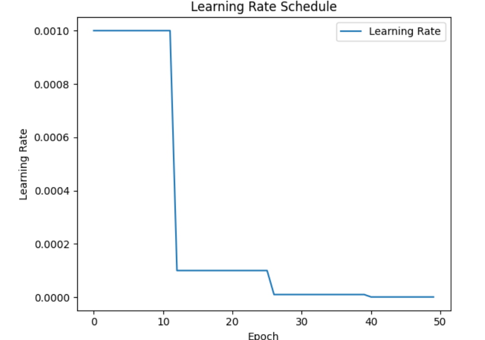
exp_lr_scheduler = lr_scheduler.StepLR(optimizer_ft, step_size=7, gamma=0.1)
> 사전 훈련된 모델 로드: 첫 번째 단계에서는 사전 훈련된 모델을 로드합니다. 여기서는 ImageNet 데이터셋으로 훈련된 ResNet18을 사용합니다.
> 마지막 완전 연결 계층 재설정: 모델의 마지막 완전 연결 계층(fc)을 새로운 작업에 맞게 조정합니다. 예를 들어, 출력 클래스의 수가 2개인 경우 nn.Linear(num_ftrs, 2)를 사용합니다. 여기서 num_ftrs는 이전 완전 연결 계층의 입력 특징 수를 나타냅니다.
> 손실 함수와 최적화 설정: 손실 함수로는 교차 엔트로피 손실(nn.CrossEntropyLoss)을 사용합니다. 최적화기(optimizer)로는 SGD(확률적 경사 하강법)를 사용하며, 학습률(learning rate)과 모멘텀(momentum)을 설정합니다.
>학습률 스케줄러 설정: 학습률 스케줄러는 학습 과정 중 학습률을 조정하는 데 사용됩니다. 여기서는 매 7 에폭(epoch)마다 학습률을 0.1의 비율로 감소시키는 StepLR 스케줄러를 사용합니다.
4. Train and evaluate
import matplotlib.pyplot as plt
def plot_training_history(train_loss_history, val_loss_history, train_accuracy_history, val_accuracy_history, lr_history):
# 2x2 서브플롯 그리드를 생성합니다
plt.figure(figsize=(12, 10))
# 훈련 및 검증 손실에 대한 첫 번째 서브플롯을 생성합니다
plt.subplot(2, 2, 1)
plt.plot(range(len(train_loss_history)), train_loss_history, label='Training Loss')
plt.plot(range(len(val_loss_history)), val_loss_history, label='Validation Loss')
plt.xlabel('Epoch')
plt.ylabel('Loss')
plt.title('Training and Validation Loss')
plt.legend()
# 훈련 및 검증 정확도에 대한 두 번째 서브플롯을 생성합니다
plt.subplot(2, 2, 2)
plt.plot(range(len(train_accuracy_history)), train_accuracy_history, label='Training Accuracy')
plt.plot(range(len(val_accuracy_history)), val_accuracy_history, label='Validation Accuracy')
plt.xlabel('Epoch')
plt.ylabel('Accuracy')
plt.title('Training and Validation Accuracy')
plt.legend()
# 학습률(Learning Rate)에 대한 세 번째 서브플롯을 생성합니다
plt.subplot(2, 2, 3)
plt.plot(range(len(lr_history)), lr_history, label='Learning Rate')
plt.xlabel('Epoch')
plt.ylabel('Learning Rate')
plt.title('Learning Rate Schedule')
plt.legend()
# 전체 그래프에 제목 추가
plt.suptitle('Training Curves', fontsize=16)
plt.tight_layout()
plt.show()
# 학습 진행
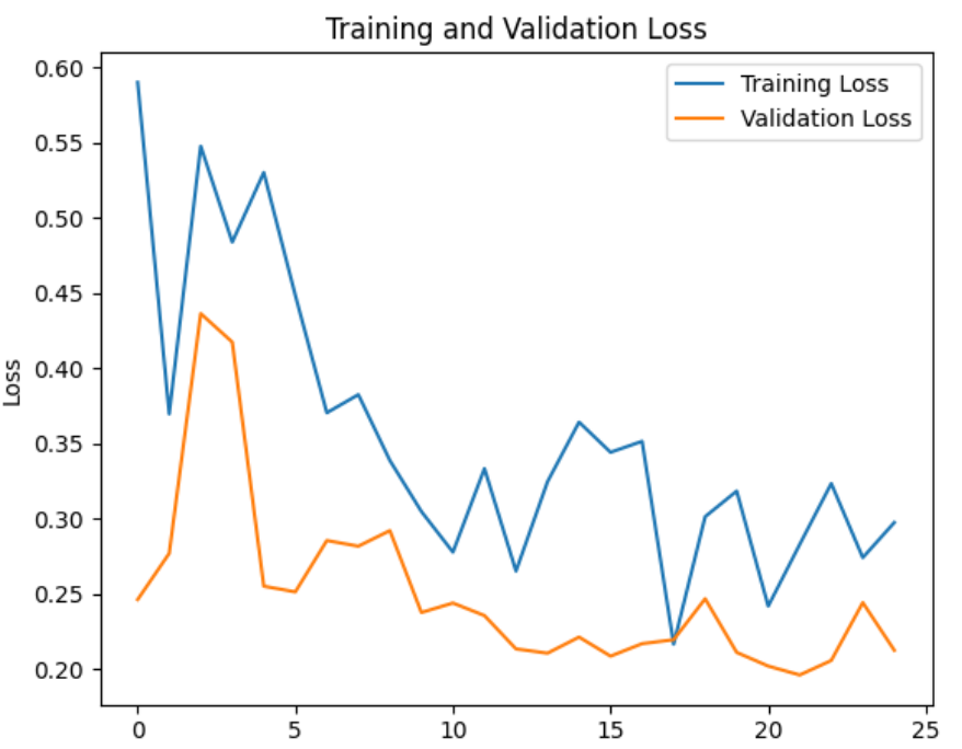
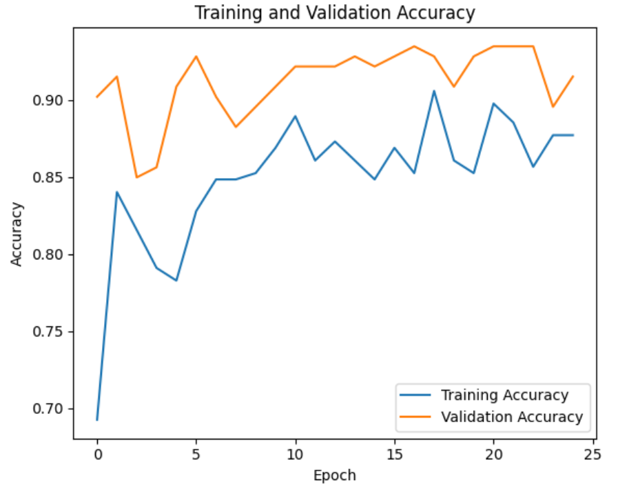
model_ft = train_model(model_ft, criterion, optimizer_ft, exp_lr_scheduler, num_epochs=25)결과(Best val Acc: 0.9346)
early stop일 경우
import torch
import torch.optim as optim
import matplotlib.pyplot as plt

# Initialize lists to track metrics
lr_history = []
train_loss_history = []
val_loss_history = []
train_accuracy_history = []
val_accuracy_history = []

# Specify the number of epochs and early stopping parameters
num_epochs = 25
early_stopping_patience = 10
early_stopping_counter = 0
best_val_loss = float('inf')
exp_lr_scheduler = lr_scheduler.StepLR(optimizer_ft, step_size=7, gamma=0.1)

for epoch in range(num_epochs):
    model_ft.train()
    running_loss = 0.0
    correct = 0
    total = 0

    for inputs, labels in dataloaders['train']:
        inputs, labels = inputs.to(device), labels.to(device)

        optimizer_ft.zero_grad()

        # Forward pass
        outputs = model_ft(inputs)
        loss = criterion(outputs, labels)

        # Backward pass and optimization
        loss.backward()
        optimizer_ft.step()

        running_loss += loss.item() * inputs.size(0)

        # Calculate accuracy
        _, predicted = torch.max(outputs, 1)
        total += labels.size(0)
        correct += (predicted == labels).sum().item()

    # Calculate training loss and accuracy
    train_loss = running_loss / dataset_sizes['train']
    train_accuracy = correct / total

    # Record learning rate, training loss, and accuracy
    lr_history.append(optimizer_ft.param_groups[0]['lr'])
    train_loss_history.append(train_loss)
    train_accuracy_history.append(train_accuracy)

    # Validation loop
    model_ft.eval()
    val_loss = 0.0
    val_correct = 0
    val_total = 0

    with torch.no_grad():
        for inputs, labels in dataloaders['val']:
            inputs, labels = inputs.to(device), labels.to(device)

            # Forward pass
            outputs = model_ft(inputs)
            loss = criterion(outputs, labels)

            val_loss += loss.item() * inputs.size(0)

            # Calculate accuracy
            _, predicted = torch.max(outputs, 1)
            val_total += labels.size(0)
            val_correct += (predicted == labels).sum().item()

    # Calculate validation loss and accuracy
    val_loss = val_loss / dataset_sizes['val']
    val_accuracy = val_correct / val_total

    # Record validation loss and accuracy
    val_loss_history.append(val_loss)
    val_accuracy_history.append(val_accuracy)

    # Early stopping logic
    if val_loss < best_val_loss:
        best_val_loss = val_loss
        early_stopping_counter = 0
    else:
        early_stopping_counter += 1

    if early_stopping_counter >= early_stopping_patience:
        print(f"Early stopping triggered. Stopped at epoch {epoch}")
        break

# 2x2 subplot grid
plt.figure(figsize=(12, 10))

# Create the first subplot for the learning rate
plt.subplot(2, 2, 1)
plt.plot(range(len(lr_history)), lr_history, label='Learning Rate')
plt.xlabel('Epoch')
plt.ylabel('Learning Rate')
plt.title('Learning Rate Schedule')
plt.legend()

# Create the second subplot for training and validation loss
plt.subplot(2, 2, 2)
plt.plot(range(len(train_loss_history)), train_loss_history, label='Training Loss')
plt.plot(range(len(val_loss_history)), val_loss_history, label='Validation Loss')
plt.xlabel('Epoch')
plt.ylabel('Loss')
plt.title('Training and Validation Loss')
plt.legend()

# Create the third subplot for training and validation accuracy
plt.subplot(2, 2, 3)
plt.plot(range(len(train_accuracy_history)), train_accuracy_history, label='Training Accuracy')
plt.plot(range(len(val_accuracy_history)), val_accuracy_history, label='Validation Accuracy')
plt.xlabel('Epoch')
plt.ylabel('Accuracy')
plt.title('Training and Validation Accuracy')
plt.legend()

plt.tight_layout()
plt.show()
Stopped at epoch 14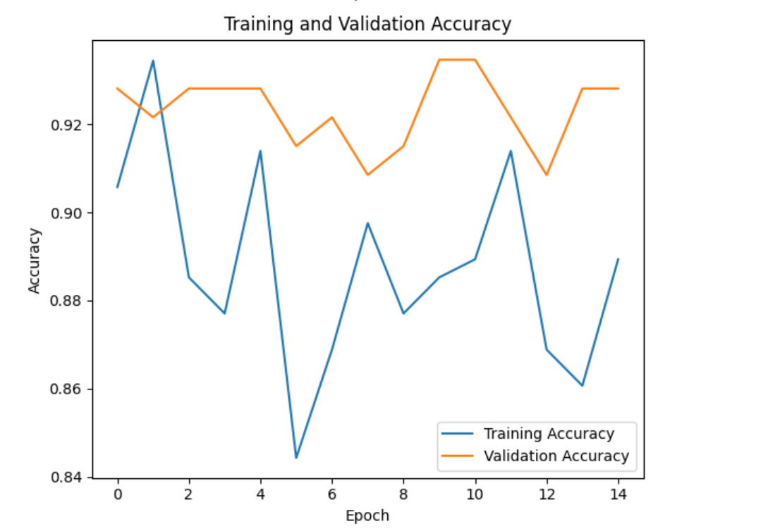
ConvNet as fixed feature extractor(고정된 특징 추출기로서의 ConvNet)
마지막 완전 연결 계층을 제외한 모든 네트워크 파라미터를 고정된다.이전에 학습한 특징 추출 계층은 동결되어 Gradien가 계산되지 않는다. 그런 다음, 마지막 완전 연결 계층을 새로운 nn.Linear 계층으로 교체하고, 이 계층의 파라미터만 학습된다. Finetuning할 계층을 선택적으로 지정하여 전체 모델을 다시 학습시키지 않고도 사용할 수 있게 한다.일부 파라미터를 동결하고 나머지 일부만 Finetuning한다
Adam Optimizer:
1. Adam은 적응형 학습률을 사용합니다. 즉, 각 매개변수에 대해 학습률이 다르며, 이는 모델 훈련 과정에서 자동으로 조정됩니다.
2. Adam은 모멘텀과 RMSprop의 개념을 결합하여, 손실 함수의 곡률을 보다 효과적으로 핸들링합니다. 이는 특히 불규칙한 데이터셋이나 복잡한 모델 구조에서 유리할 수 있습니다.
3. Adam은 보통 빠르게 수렴하며, 초반에 더 큰 학습률을 허용합니다.
SGD Optimizer:
1. SGD는 모든 매개변수에 대해 동일한 학습률을 사용합니다. 이 학습률은 학습 과정에서 수동으로 조정될 수 있습니다.
2. SGD는 더 단순하고 해석하기 쉽습니다. 때로는 너무 큰 학습률로 인해 발생할 수 있는 불안정성을 피할 수 있습니다.
3. SGD는 보통 더 많은 에포크가 필요할 수 있으며, 학습률 스케줄링에 더 민감합니다.
최적화 (Adam)
model_conv = torchvision.models.resnet18(weights='IMAGENET1K_V1')
for param in model_conv.parameters():
    param.requires_grad = False

# Parameters of newly constructed modules have requires_grad=True by default
num_ftrs = model_conv.fc.in_features
model_conv.fc = nn.Linear(num_ftrs, 2)

model_conv = model_conv.to(device)

criterion = nn.CrossEntropyLoss()

# Observe that only parameters of final layer are being optimized as
# opposed to before.
optimizer_conv = optim.Adam(model_conv.fc.parameters(), lr=0.001)
# Decay LR by a factor of 0.1 every 7 epochs
exp_lr_scheduler = lr_scheduler.StepLR(optimizer_conv, step_size=7, gamma=0.1)
Train and evaluate
import matplotlib.pyplot as plt

def plot_training_history(lr_history, train_loss_history, val_loss_history, train_accuracy_history, val_accuracy_history):
    # 2x2 subplot grid
    plt.figure(figsize=(12, 10))

    # Create the first subplot for the learning rate
    plt.subplot(2, 2, 1)
    plt.plot(range(len(lr_history)), lr_history, label='Learning Rate')
    plt.xlabel('Epoch')
    plt.ylabel('Learning Rate')
    plt.title('Learning Rate Schedule')
    plt.legend()

    # Create the second subplot for training and validation loss
    plt.subplot(2, 2, 2)
    plt.plot(range(len(train_loss_history)), train_loss_history, label='Training Loss')
    plt.plot(range(len(val_loss_history)), val_loss_history, label='Validation Loss')
    plt.xlabel('Epoch')
    plt.ylabel('Loss')
    plt.title('Training and Validation Loss')
    plt.legend()

    # Create the third subplot for training and validation accuracy
    plt.subplot(2, 2, 3)
    plt.plot(range(len(train_accuracy_history)), train_accuracy_history, label='Training Accuracy')
    plt.plot(range(len(val_accuracy_history)), val_accuracy_history, label='Validation Accuracy')
    plt.xlabel('Epoch')
    plt.ylabel('Accuracy')
    plt.title('Training and Validation Accuracy')
    plt.legend()

    plt.tight_layout()
    plt.show()

model_conv = train_model(model_conv, criterion, optimizer_conv,exp_lr_scheduler, num_epochs=25)
Best val Acc: 0.9608
최적화 (SGD)인 경우에는
Best val Acc: 0.9412
즉, Adam이 Sgd보다 더 나은 성능을 보여준다.
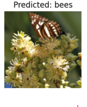
custom images
'AI기초프로젝트 과제' 카테고리의 다른 글
| AI기초프로젝트 3주차 과제 - Naver Shopping Review Sentiment Analysis (0) | 2023.11.06 |
|---|---|
| 기말 프로젝트 (0) | 2023.11.06 |
| AI기초프로젝트 5주차 과제 - 감성Fine-tuning (0) | 2023.10.22 |
| AI기초프로젝트 2주차 과제 - Detectron2 (0) | 2023.10.17 |
| AI기초프로젝트 1주차 과제 - 음성인식 (0) | 2023.10.17 |


