1. Colab에 Mecab 설치
여기서는 형태소 분석기 Mecab을 사용합니다. 저자의 경우 Mecab을 편하게 사용하기 위해서 구글의 Colab을 사용하였습니다. 참고로 Colab에서 실습하는 경우가 아니라면 아래의 방법으로 Mecab이 설치되지 않습니다. 이 경우 해당 환경에 맞게 Mecab을 설치하시거나 다른 형태소 분석기를 사용하시기 바랍니다.
# Colab에 Mecab 설치/ 형태소 분석기 Mecab을 사용
!pip install konlpy
!pip install mecab-python
!bash <(curl -s https://raw.githubusercontent.com/konlpy/konlpy/master/scripts/mecab.sh)
| Mecab : 일본어 형태소 분석기로, 오픈 소스 프로젝트입니다. 원래 일본어 텍스트 처리를 위해 만들어졌지만, 한국어 처리를 위한 사전과 함께 한국어 형태소 분석기로도 널리 사용됩니다. Mecab은 텍스트를 형태소로 분리하고, 각 형태소의 기본형, 품사 등을 태깅하는 기능을 제공합니다. CRF(Conditional Random Fields) 알고리즘을 사용하여 각 형태소의 경계를 찾고, 품사를 할당합니다. 이는 높은 정확도로 텍스트의 형태소를 분석할 수 있게 해주며, 특히 일본어와 한국어와 같이 복잡한 굴절을 가진 언어에서 강력한 성능을 발휘합니다. |
2. 네이버 쇼핑 리뷰 데이터에 대한 이해와 전처리
import re
import pandas as pd
import numpy as np
import matplotlib.pyplot as plt
import urllib.request from collections
import Counter from konlpy.tag
import Mecab from sklearn.model_selection
import train_test_split from tensorflow.keras.preprocessing.text
import Tokenizer from tensorflow.keras.preprocessing.sequence
import pad_sequences
1) 데이터 로드하기
urllib.request.urlretrieve("https://raw.githubusercontent.com/bab2min/corpus/master/sentiment/naver_shopping.txt", filename="ratings_total.
2) 훈련 데이터와 테스트 데이터 분리하기
현재 갖고 있는 데이터는 레이블을 별도로 갖고있지 않습니다. 평점이 4, 5인 리뷰에는 레이블 1을, 평점이 1, 2인 리뷰에는 레이블 0을 부여합니다. 부여된 레이블은 새로 생성한 label이라는 열에 저장합니다.
total_data['label'] = np.select([total_data.ratings > 3], [1], default=0) total_data[:5]

(4, 199908, 2)총 샘플의 수 : 199908
False
훈련용 리뷰의 개수 : 149931
테스트용 리뷰의 개수 : 49977
3) 레이블의 분포 확인
<Axes: > label count
0 0 74918
1 1 75013
4) 데이터 정제하기
<ipython-input-13-7fd6903b4870>:2: FutureWarning: The default value of regex will change from True to False in a future version.
  train_data['reviews'] = train_data['reviews'].str.replace("[^ㄱ-ㅎㅏ-ㅣ가-힣 ]","")
ratings    0
reviews    0
label      0
dtype: int64
전처리 후 테스트용 샘플의 개수 : 49977
<ipython-input-14-2e4409826f1a>:3: FutureWarning: The default value of regex will change from True to False in a future version.
  test_data['reviews'] = test_data['reviews'].str.replace("[^ㄱ-ㅎㅏ-ㅣ가-힣 ]","") # 정규 표현식 수행
5) 토큰화
['와', '이런', '것', '도', '상품', '이', '라고', '차라리', '내', '가', '만드', '는', '게', '나을', '뻔']
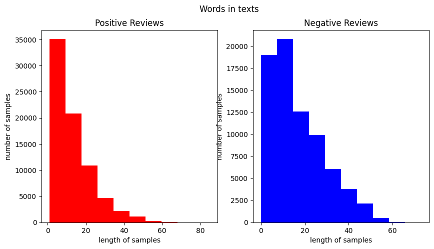
6) 단어와 길이 분포 확인하기
[('네요', 31802), ('는데', 20197), ('안', 19719), ('어요', 14838), ('있', 13200), ('너무', 13057), ('했', 11766), ('좋', 9803), ('배송', 9677), ('같', 8997), ('어', 8929), ('구매', 8869), ('거', 8861), ('없', 8672), ('아요', 8640), ('습니다', 8436), ('그냥', 8355), ('되', 8345), ('잘', 8029), ('않', 7985)]
[('좋', 39422), ('아요', 21186), ('네요', 19894), ('어요', 18673), ('잘', 18603), ('구매', 16165), ('습니다', 13320), ('있', 12391), ('배송', 12274), ('는데', 11635), ('합니다', 9801), ('했', 9783), ('먹', 9640), ('재', 9274), ('너무', 8398), ('같', 7867), ('만족', 7259), ('거', 6484), ('어', 6330), ('쓰', 6291)]
긍정 리뷰의 평균 길이 : 13.579646194659592
부정 리뷰의 평균 길이 : 17.03148775995088
7) 정수 인코딩
기계가 텍스트를 숫자로 처리할 수 있도록 훈련 데이터와 테스트 데이터에 정수 인코딩을 수행해야 합니다. 훈련 데이터에 대해서 단어 집합(vocaburary)을 만들어봅시다
단어 집합(vocabulary)의 크기 : 40127
등장 빈도가 1번 이하인 희귀 단어의 수: 18275
단어 집합에서 희귀 단어의 비율: 45.5429012884093
전체 등장 빈도에서 희귀 단어 등장 빈도 비율: 0.7964299021840265
단어가 약 40,000개가 존재합니다. 등장 빈도가 threshold 값인 2회 미만. 즉, 1회인 단어들은 단어 집합에서 약 45%를 차지합니다. 하지만, 실제로 훈련 데이터에서 등장 빈도로 차지하는 비중은 매우 적은 수치인 약 0.8%밖에 되지 않습니다. 아무래도 등장 빈도가 1회인 단어들은 자연어 처리에서 중요하지 않을 것으로 저자는 판단했습니다. 이 단어들은 정수 인코딩 과정에서 배제시키겠습니다. 등장 빈도수가 1인 단어들의 수를 제외한 단어의 개수를 단어 집합의 최대 크기로 제한합니다.
단어 집합의 크기 : 21854
[[67, 2060, 300, 14294, 263, 73, 6, 237, 168, 136, 801, 2940, 626, 2, 76, 62, 207, 40, 1344, 155, 3, 6], [482, 400, 52, 8525, 2592, 2450, 338, 2941, 251, 2351, 39, 473, 2], [45, 24, 832, 104, 35, 2366, 160, 7, 10, 8058, 4, 1319, 30, 138, 323, 44, 59, 160, 138, 7, 1916, 2, 113, 163, 1385, 307, 119, 135]]
8) 패딩
서로 다른 길이의 샘플들의 길이를 동일하게 맞춰주는 패딩 작업을 진행해보겠습니다. 전체 데이터에서 가장 길이가 긴 리뷰와 전체 데이터의 길이 분포를 알아보겠습니다.
[[14, 704, 767, 115, 186, 252, 12], [338, 3907, 62, 3819, 1624], [11, 69, 2, 49, 164, 3, 27, 15, 6, 514, 289, 17, 92, 110, 584, 59, 7, 2]]
리뷰의 최대 길이 : 85
리뷰의 평균 길이 : 15.304473391093236
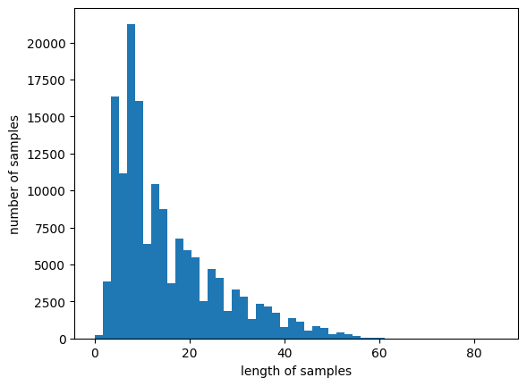
전체 샘플 중 길이가 80 이하인 샘플의 비율: 99.99933302652553
3. GRU로 네이버 쇼핑 리뷰 감성 분류하기
EarlyStopping(monitor='val_loss', mode='min', verbose=1, patience=4)는 검증 데이터 손실(val_loss)이 증가하면, 과적합 징후므로 검증 데이터 손실이 4회 증가하면 정해진 에포크가 도달하지 못하였더라도 학습을 조기 종료(Early Stopping)한다는 의미입니다. ModelCheckpoint를 사용하여 검증 데이터의 정확도(val_acc)가 이전보다 좋아질 경우에만 모델을 저장합니다. validation_split=0.2을 사용하여 훈련 데이터의 20%를 검증 데이터로 분리해서 사용하고, 검증 데이터를 통해서 훈련이 적절히 되고 있는지 확인합니다. 검증 데이터는 기계가 훈련 데이터에 과적합되고 있지는 않은지 확인하기 위한 용도로 사용됩니다.
from tensorflow.keras.layers import Embedding, Dense, GRU
from tensorflow.keras.models import Sequential
from tensorflow.keras.models import load_model
from tensorflow.keras.callbacks import EarlyStopping, ModelCheckpoint
embedding_dim = 100
hidden_units = 128
model = Sequential()
model.add(Embedding(vocab_size, embedding_dim))
model.add(GRU(hidden_units))
model.add(Dense(1, activation='sigmoid'))
es = EarlyStopping(monitor='val_loss', mode='min', verbose=1, patience=4)
mc = ModelCheckpoint('best_model.h5', monitor='val_acc', mode='max', verbose=1, save_best_only=True)
model.compile(optimizer='rmsprop', loss='binary_crossentropy', metrics=['acc'])
history = model.fit(X_train, y_train, epochs=15, callbacks=[es, mc], batch_size=64, validation_split=0.2)
Epoch 8/15
1875/1875 [==============================] - ETA: 0s - loss: 0.1525 - acc: 0.9492
Epoch 8: val_acc did not improve from 0.92360
1875/1875 [==============================] - 12s 6ms/step - loss: 0.1525 - acc: 0.9492 - val_loss: 0.2232 - val_acc: 0.9202
Epoch 9/15
1875/1875 [==============================] - ETA: 0s - loss: 0.1436 - acc: 0.9524
Epoch 9: val_acc did not improve from 0.92360
1875/1875 [==============================] - 12s 6ms/step - loss: 0.1436 - acc: 0.9524 - val_loss: 0.2316 - val_acc: 0.9177
Epoch 9: early stopping
import matplotlib.pyplot as plt
# 훈련 손실 및 정확도
train_loss = history.history['loss'] train_acc = history.history['acc']
# 검증 손실 및 정확도
val_loss = history.history['val_loss'] val_acc = history.history['val_acc']
# 에포크 수
epochs = range(1, len(train_loss) + 1)
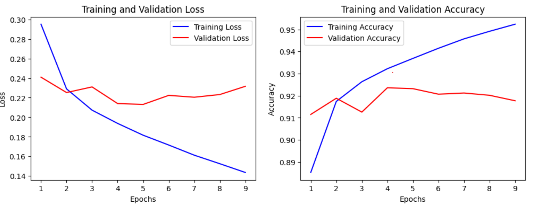
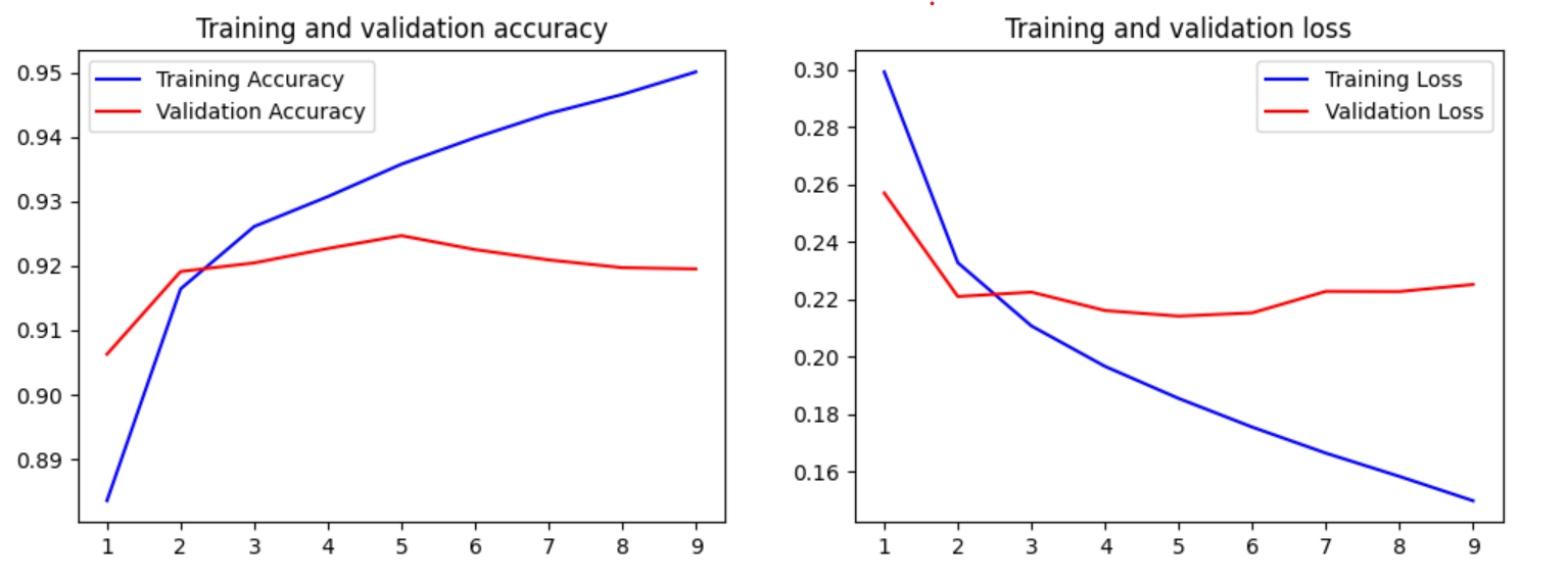
# 손실 그래프 plt.figure(figsize=(12, 4)) plt.subplot(1, 2, 1) plt.plot(epochs, train_loss, 'b', label='Training Loss') plt.plot(epochs, val_loss, 'r', label='Validation Loss') plt.title('Training and Validation Loss') plt.xlabel('Epochs') plt.ylabel('Loss') plt.legend()
# 정확도 그래프
plt.subplot(1, 2, 2) plt.plot(epochs, train_acc, 'b', label='Training Accuracy') plt.plot(epochs, val_acc, 'r', label='Validation Accuracy') plt.title('Training and Validation Accuracy') plt.xlabel('Epochs') plt.ylabel('Accuracy') plt.legend() plt.show()
1562/1562 [==============================] - 5s 3ms/step - loss: 0.2186 - acc: 0.9221

 테스트 정확도: 0.9221
EarlyStopping 안할경우(GRU)
from tensorflow.keras.layers import Embedding, Dense, GRU
from tensorflow.keras.models import Sequential
embedding_dim = 100
hidden_units = 128
model = Sequential()
model.add(Embedding(vocab_size, embedding_dim))
model.add(GRU(hidden_units))
model.add(Dense(1, activation='sigmoid'))
model.compile(optimizer='rmsprop', loss='binary_crossentropy', metrics=['acc'])
model.fit(X_train, y_train, epochs=15, batch_size=64, validation_split=0.2)
import matplotlib.pyplot as plt
# 훈련 손실 및 정확도
train_loss = model.history.history['loss'] train_acc = model.history.history['acc']
# 검증 손실 및 정확도
val_loss = model.history.history['val_loss'] val_acc = model.history.history['val_acc']
# 에포크 수
epochs = range(1, len(train_loss) + 1)
# 손실 그래프
plt.figure(figsize=(12, 4)) plt.subplot(1, 2, 1) plt.plot(epochs, train_loss, 'b', label='Training Loss') plt.plot(epochs, val_loss, 'r', label='Validation Loss') plt.title('Training and Validation Loss') plt.xlabel('Epochs') plt.ylabel('Loss') plt.legend()
# 정확도 그래프
plt.subplot(1, 2, 2) plt.plot(epochs, train_acc, 'b', label='Training Accuracy') plt.plot(epochs, val_acc, 'r', label='Validation Accuracy') plt.title('Training and Validation Accuracy') plt.xlabel('Epochs') plt.ylabel('Accuracy') plt.legend() plt.show()
Epoch 14/15
1875/1875 [==============================] - 12s 6ms/step - loss: 0.1044 - acc: 0.9658 - val_loss: 0.2876 - val_acc: 0.9120
Epoch 15/15
1875/1875 [==============================] - 12s 6ms/step - loss: 0.0976 - acc: 0.9678 - val_loss: 0.3007 - val_acc: 0.9068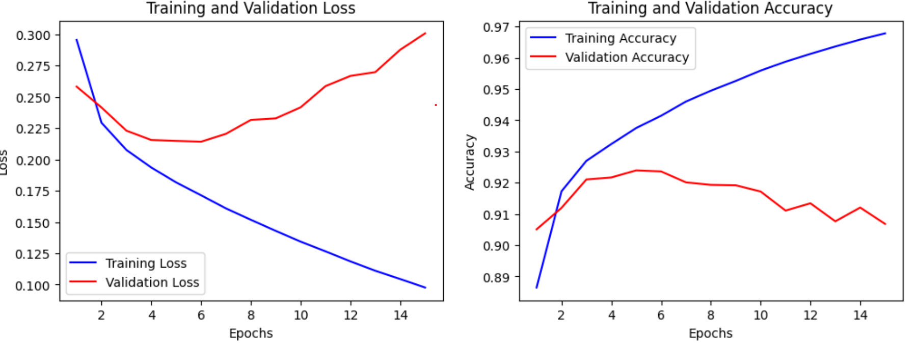
(1) EarlyStopping했을 때,
Epoch 9: val_acc did not improve from 0.92360: 이전 에포크에서 달성한 가장 높은 검증 정확도는 92.36%였으며, 현재 에포크에서는 이보다 개선되지 않았습니다.
(2) EarlyStopping안했을 때,
Epoch 15/15 loss: 0.0976 - acc: 0.9678 - val_loss: 0.3007 - val_acc: 0.9068
따라서, 이 모델은 검증 데이터셋에서 약 90.68%의 정확도를 달성했다
> 즉, EarlyStopping했을 때 , 더 나은 결과를 보여주고있다
LSTM로 네이버 쇼핑 리뷰 감성 분류하기
Epoch 9: val_acc did not improve
loss: 0.1497 - acc: 0.9501 - val_loss: 0.2251 - val_acc: 0.9195
Epoch 9: early stopping
LSTM / GRU
> Gru인 경우 ( Epoch 9: val_acc did not improve from 0.92360) 92%의 정학도가 찍혔으며 9에포크에서 학습이 조기중단되었다
> Lstm인 경우 ( Epoch 9: val_acc did not improve from 0.92467) 92%의 정확도로 Gru와 비슷하게 찍혔으며 얼리스탑을 걸었을때도 비슷하게 9에포크에서 학습이 중단되었다
4. 리뷰 예측해보기
임의의 문장에 대한 예측을 위해서는 학습하기 전 전처리를 동일하게 적용해줍니다.
전처리의 순서: 정규 표현식을 통한 한국어 외 문자 제거 -> 토큰화, 불용어 제거 ->정수 인코딩 -> 패딩
1/1 [==============================] - 0s 323ms/step
96.68% 확률로 긍정 리뷰입니다.
1/1 [==============================] - 0s 21ms/step
99.65% 확률로 부정 리뷰입니다.
'AI기초프로젝트 과제' 카테고리의 다른 글
| 기말 프로젝트 (0) | 2023.11.06 |
|---|---|
| AI기초프로젝트 5주차 과제 - 감성Fine-tuning (0) | 2023.10.22 |
| AI기초프로젝트 4주차 과제 - Transfer Learning for Computer Vision Tutorial (0) | 2023.10.22 |
| AI기초프로젝트 2주차 과제 - Detectron2 (0) | 2023.10.17 |
| AI기초프로젝트 1주차 과제 - 음성인식 (0) | 2023.10.17 |


